bet_sizing

A classifier that is right 55% of the time can still lose money if it bets the same amount on a 51% call as on a 90% one. AFML Chapter 10 opens with the poker version of the point: the cards are the forecast, and the money is made or lost in how the hand is bet. This module is the step between a prediction and an order. It offers three routes, depending on what the model produces:

You have	Use	AFML
a class probability (typically from a meta-label model)	`bet_size_probability`	§10.3–10.5
a price forecast and the current market price	`bet_size_dynamic`	§10.6
only the sides and lifespans of the bets	`bet_size_budget`, `bet_size_reserve`	§10.2

From a probability

Under the null hypothesis that the model knows nothing, the predicted class has probability $1/K$ . The size is how far the prediction is from that, as a test statistic pushed through the normal CDF (Snippet 10.1):

z = \frac{p - 1/K}{\sqrt{p\,(1-p)}}, \qquad m = s\,\bigl(2\Phi(z) - 1\bigr)

where $p$ is the probability of the predicted class, $K$ the number of classes and $s$ the side. $m$ lies in $[-1, 1]$ : a fraction of the maximum position. get_signal is exactly this; with pred omitted it returns the unsigned size.

Two further steps make it tradeable. Signals stay alive until their label’s end time, so at any moment several are open; avg_active_signals replaces each with the mean of the signals live at that instant (§10.4), which stops the position from flipping every time a new one arrives. Then discrete_signal rounds to a step (§10.5), so that a change from 0.337 to 0.328 does not generate an order. bet_size_probability runs all three.

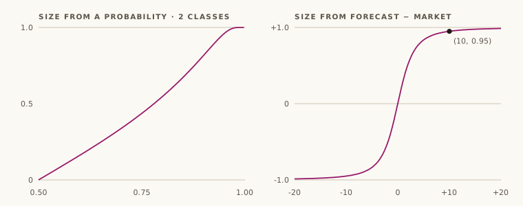
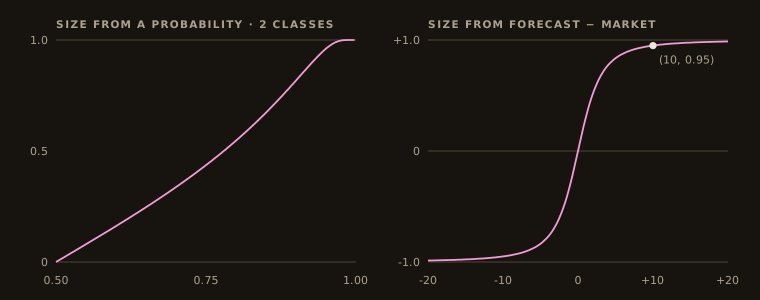
Two curves. Left: bet size against predicted probability for a two-class model, rising from zero at a probability of one half, nearly linearly at first, and saturating at one as the probability approaches one. Right: bet size against the gap between forecast and market price, an S-shaped curve through zero that passes through 0.95 at a gap of ten. — The two sizing functions. Left: `get_signal` with two classes. Right: the sigmoid that `bet_size_dynamic` uses, with its fixed calibration point.

from openquant import bet_sizing

# 1. Probability -> size. A two-class meta-label model: 0.5 is "no idea".
probs = [0.50, 0.55, 0.60, 0.70, 0.80, 0.90, 0.99]
sizes = bet_sizing.get_signal(probs, 2)
print("p    ", "  ".join(f"{p:5.2f}" for p in probs))
print("size ", "  ".join(f"{m:5.2f}" for m in sizes))

# 2. Bets overlap. Four signals, each alive for two hours; the side comes from the primary model.
starts = [f"2024-01-02 {h:02d}:00:00" for h in (9, 10, 11, 14)]
ends = [f"2024-01-02 {h:02d}:00:00" for h in (11, 12, 13, 16)]
p, side = [0.70, 0.90, 0.60, 0.80], [1.0, 1.0, -1.0, -1.0]

alone = bet_sizing.bet_size_probability(starts, ends, p, side, 2, 0.0, False)
averaged = bet_sizing.bet_size_probability(starts, ends, p, side, 2, 0.0, True)
stepped = bet_sizing.bet_size_probability(starts, ends, p, side, 2, 0.1, True)
print()
print("each signal alone:", [round(v, 3) for _, v in alone])
for (t, avg), (_, step) in zip(averaged, stepped):
    print(f"{t[11:16]}  average of live bets {avg:+.3f}  in steps of 0.1 {step:+.1f}")

# 3. A price forecast instead of a probability: how many of 100 contracts to hold, and the
#    worst price at which moving to that position is still justified.
print()
for market in (99.0, 95.0, 90.0):
    size, target, limit = bet_sizing.bet_size_dynamic([0.0], [100.0], [market], [100.0])[0]
    print(f"forecast 100, market {market:5.1f}: size {size:.3f}, hold {target:3.0f}, limit {limit:.2f}")

p      0.50   0.55   0.60   0.70   0.80   0.90   0.99
size   0.00   0.08   0.16   0.34   0.55   0.82   1.00

each signal alone: [0.337, 0.818, -0.162, -0.547]
09:00  average of live bets +0.337  in steps of 0.1 +0.3
10:00  average of live bets +0.578  in steps of 0.1 +0.6
11:00  average of live bets +0.328  in steps of 0.1 +0.3
12:00  average of live bets -0.162  in steps of 0.1 -0.2
13:00  average of live bets +0.000  in steps of 0.1 +0.0
14:00  average of live bets -0.547  in steps of 0.1 -0.5
16:00  average of live bets +0.000  in steps of 0.1 +0.0

forecast 100, market  99.0: size 0.291, hold  29, limit 99.50
forecast 100, market  95.0: size 0.836, hold  83, limit 98.22
forecast 100, market  90.0: size 0.950, hold  95, limit 97.57

The first table is the shape of the function: a 55% call earns an 8% position and a 70% call a third. It is cautious where most classifiers live, and a model whose probabilities are not calibrated will be sized wrongly by exactly the amount of its miscalibration — calibrate before sizing.

The second shows what averaging is for. At 11:00 the 0.70 long has expired, and a new short at −0.162 arrives while the 0.90 long is still open: the book moves to +0.328, not to −0.162. At 13:00 nothing is live and the position is flat. Note the rounding at 12:00: −0.162 becomes −0.2, because the step rounds to nearest, not toward zero.

From a price forecast

When the model forecasts a price $f$ rather than a probability, size should grow with the gap to the market price $p$ and saturate (§10.6). With $x = f - p$ :

m(x) = \frac{x}{\sqrt{w + x^{2}}}, \qquad \hat q = \operatorname{trunc}\bigl(m(x)\,Q\bigr), \qquad L = \frac{1}{n}\sum_{i=1}^{n} \Bigl(f - \tfrac{k_i}{Q}\sqrt{\tfrac{w}{1-(k_i/Q)^{2}}}\Bigr), \qquad k_i = q + i\,\operatorname{sgn}(\hat q - q),\quad n = \lvert \hat q - q\rvert

$\hat q$ is the target position out of a maximum $Q$ , $q$ the current one, and $L$ the limit price: the average, over each position $k_i$ passed through on the way from $q$ to $\hat q$ , of the price at which holding $k_i$ units is exactly justified. Buying above $L$ means paying more for the marginal units than the forecast supports. In the example, with the market at 95 and a forecast of 100, the target is 83 contracts and the order should not be filled above 98.22. Both positions are truncated to whole units, and $L$ is NaN when they are equal.

Where this departs from Snippet 10.4

Snippet 10.4 loops over j in range(abs(pos + sgn), abs(tPos + 1)) with unsigned j and divides by tPos - pos. When the position is long and growing ( $0 \le q < \hat q$ ) that is exactly the sum above, and the two agree. In every other direction the book’s loop does not follow the move, so openquant uses the path $k_1, \dots, k_n$ with signs kept:

Move (with $Q = 10$ )	Positions averaged here	Snippet 10.4 as written
0 → 4 (increasing a long)	1, 2, 3, 4	the same
10 → 5 (reducing a long)	9, 8, 7, 6, 5	none: the range is empty, $L = 0$
0 → −4 (going short)	−1, −2, −3, −4	$j = 1, 2$ (the bound is `abs(tPos + 1)` = 3), unsigned, divided by −4
3 → −2 (crossing zero)	2, 1, 0, −1, −2	none: the range from 2 to 1 is empty

Keeping the sign matters: a short’s limit price lies above $f$ , the mirror image of a long’s below it, and at $k = 0$ the term is $f$ itself. Until issue #163 openquant used the book’s unsigned loop with abs(tPos) as the upper bound, so it returned 0 when reducing, the long’s price for a short, and 19.96 for the 3 → −2 move on the power curve with $w = 1$ and $f = 100$ (now 100). bet_size_dynamic computes its limit column the same way.

bet_size_dynamic fixes $w$ . It calibrates the curve so that a divergence of 10 price units gives a size of 0.95 — get_w_sigmoid(10.0, 0.95) — and there is no argument to change it. Ten units is a large gap for a stock at 20 and nothing for an index at 5,000, so for anything other than a first look, calibrate your own: get_w(divergence, size, "sigmoid"), then get_target_pos and limit_price with that $w$ . The "power" variants use $m(x)=\operatorname{sgn}(x)\lvert x\rvert^{w}$ and require the divergence to be scaled into $[-1, 1]$ ; outside it they return BetSizingError::PriceDivergenceOutOfRange.

From concurrency alone

§10.2 sizes without any model output, from how many bets are open. With $L_t$ and $S_t$ the number of concurrent long and short bets at $t$ , and $c_t = L_t - S_t$ :

m_t^{\text{budget}} = \frac{L_t}{\max_s L_s} - \frac{S_t}{\max_s S_s}, \qquad m_t^{\text{reserve}} = \begin{cases} \dfrac{F(c_t) - F(0)}{1 - F(0)} & c_t \ge 0 \\[8pt] \dfrac{F(c_t) - F(0)}{F(0)} & c_t < 0 \end{cases}

bet_size_budget is the first: it reaches full size only when concurrency is at its historical maximum, which keeps capacity in reserve for the moment signals pile up. bet_size_reserve is the second, with $F$ the CDF of a mixture of two Gaussians fitted to $c_t$ . bet_size_reserve_full fits that mixture by EM from random starting points, so its output changes from run to run; fit once, keep the five parameters [mu1, mu2, sigma1, sigma2, p1], and pass them to bet_size_reserve for reproducible sizes. The maxima in the budget formula are taken over the sample you pass in, so computing it on a full backtest and trading on it looks ahead.

From Rust

use openquant::bet_sizing::{get_signal, get_target_pos, get_w, limit_price, BetSizingError};

// Probability to size: no edge at 1/K, saturating towards 1.
let sizes = get_signal(&[0.5, 0.7, 0.9], 2, None);
assert!(sizes[0].abs() < 1e-12);
assert!((sizes[1] - 0.3374).abs() < 1e-4 && (sizes[2] - 0.8176).abs() < 1e-4);

// Calibrate the sigmoid for this instrument: a gap of 2.0 should be a 0.9 bet.
let w = get_w(2.0, 0.9, "sigmoid")?;
let target = get_target_pos(w, 101.5, 100.0, 50.0, "sigmoid")?; // forecast, market, max position
let limit = limit_price(target, 0.0, 101.5, w, 50.0, "sigmoid")?;
assert_eq!(target, 42.0);
assert!(limit > 100.0 && limit < 101.5);

// An unknown function name is an error, not a panic.
assert!(matches!(get_w(2.0, 0.9, "logistic"), Err(BetSizingError::InvalidFunction { .. })));

What to watch for

$p$ is the probability that the bet is right. With a meta-label model and a side from a primary model, as in the example, that is the model’s $p_1$ : above $1/K$ it sizes the primary model’s call, and below $1/K$ the size goes negative — a bet against the primary model, not a smaller bet with it. If you only ever want to follow or stand aside, floor the size at zero yourself.
$p$ of exactly 0 or 1 divides by zero. The result is $\pm\infty$ in $z$ and a size of exactly $\pm 1$ ; clip probabilities if your model emits hard 0s and 1s.
A signal is live on $[t_0, t_1)$ . At its own end time it no longer counts, which is why 13:00 and 16:00 in the example are flat.
A step_size of zero or less disables discretisation rather than raising.
bet_size_dynamic broadcasts. Each of its four inputs must have length 1 or the common length; anything else is BetSizingError::ShapeMismatch.
Timestamps from Python are strings, "%Y-%m-%d %H:%M:%S" with an optional fractional second. Output times keep the fraction, written as str(datetime) writes it.

labeling — meta-labels are what the probability model is trained on, and each label’s end time is the lifespan of its bet.
sampling — the same concurrency, used to weight observations.
risk-metrics and strategy-risk — what the sized strategy then has to survive.
ef3m — the moment-matching mixture fit AFML uses for the reserve method; this module fits by EM instead.

API reference

Python

Signatures, parameters, return values and errors for every function: openquant.bet_sizing.

bet_sizing.get_signal — Convert predicted-class probabilities into bet sizes in `[-1, 1]`.
bet_sizing.avg_active_signals — Average the signals that are live at each change point.
bet_sizing.discrete_signal — Round bet sizes to multiples of `step_size` and clamp them to `[-1, 1]`.
bet_sizing.bet_size_probability — Size bets from classifier probabilities.
bet_sizing.bet_size_dynamic — Dynamic bet sizing from a price forecast.
bet_sizing.bet_size_budget — Budgeting bet size `L_t / max(L) - S_t / max(S)` from concurrent bet counts.
bet_sizing.bet_size_reserve — Reserve bet sizes under a given two-Gaussian mixture fit.
bet_sizing.bet_size_reserve_full — Reserve bet sizing with a two-Gaussian mixture fitted to the net concurrency.

Rust

Rustdoc for this commit, with every public item of openquant::bet_sizing (after a crates.io release the same pages are on docs.rs):