strategy_risk

Portfolio risk is about the holdings: how much can these positions lose. Strategy risk (AFML Chapter 15) is about the process that produces them: what is the chance that this strategy, run as designed, fails to deliver the Sharpe ratio it was funded for. The chapter’s observation is that a strategy can be described by three numbers — how often it bets, how often it is right, and what it wins and loses — and that its Sharpe ratio is a steep function of the second one. A strategy that needs 55% precision and delivers 53% has not underperformed slightly. It has failed.

Bets as coin flips

Model each bet as an independent draw that pays $\pi_+$ with probability $p$ and $\pi_-$ otherwise, $n$ times a year. With symmetric payouts, $\pi_+=-\pi_-$ , the payout size cancels and the annualised Sharpe ratio is (§15.2)

\theta \;=\; \frac{2p-1}{2\sqrt{p(1-p)}}\,\sqrt{n}

With asymmetric payouts (§15.3),

\theta \;=\; \frac{(\pi_+-\pi_-)\,p+\pi_-}{(\pi_+-\pi_-)\sqrt{p(1-p)}}\,\sqrt{n}

Each formula can be solved for any one of its variables. sharpe_* computes $\theta$ ; implied_precision_* the $p$ needed for a target $\theta$ at a given $n$ ; implied_frequency_* the $n$ needed at a given $p$ . The asymmetric precision is the root of a quadratic, and the function returns the smallest root in $[0,1]$ that reaches the target.

The probability of failing

Precision is not known; it is estimated from a finite record. §15.4 turns that into a probability. From the record of bet outcomes, take $\pi_+$ and $\pi_-$ as the mean win and mean loss and $n$ as bets per year, and solve for $p^*$ , the precision below which the target Sharpe ratio is missed. Then bootstrap: draw $n\times$ investor_horizon_years outcomes with replacement, record the share of winners, repeat. The share of bootstrap precisions at or below $p^*$ is the probability of failure. estimate_strategy_failure_probability returns that figure (empirical_failure_probability), the same read from a Gaussian kernel density fitted to the bootstrap sample (kde_failure_probability), and the inputs it derived. AFML’s guidance is that a strategy with a failure probability above 5% is too risky to run, however good its backtest.

import random

from openquant import strategy_risk as sr

# How precise must a strategy be to reach an annualised Sharpe ratio of 2?
print("bets/year   symmetric payout   wins +1% / loses -2%")
for n in (12, 52, 260, 2600):
    sym = sr.implied_precision_symmetric(2.0, n)
    asym = sr.implied_precision_asymmetric(2.0, n, 0.01, -0.02)
    print(f"{n:9d}   {sym:16.3f}   {asym:20.3f}")

# A two-year record of 520 bets: 70% win +1%, 30% lose -2%. Expected value per bet: +0.1%.
rng = random.Random(12)
bets = [0.01 if rng.random() < 0.70 else -0.02 for _ in range(520)]
report = sr.estimate_strategy_failure_probability(bets, years_elapsed=2.0, target_sharpe=1.0,
                                                  investor_horizon_years=2.0, seed=5)
print(f"observed precision {sum(b > 0 for b in bets) / len(bets):.3f}, "
      f"needed for Sharpe 1: {report['implied_precision_threshold']:.3f}")
print(f"probability of falling short over the next two years: "
      f"{report['empirical_failure_probability']:.2f}")

bets/year   symmetric payout   wins +1% / loses -2%
       12              0.750                  0.864
       52              0.634                  0.781
      260              0.562                  0.722
     2600              0.520                  0.685
observed precision 0.721, needed for Sharpe 1: 0.695
probability of falling short over the next two years: 0.10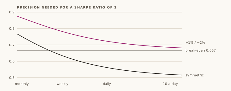

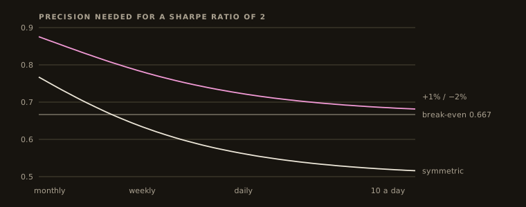
Precision needed for an annualised Sharpe ratio of 2, against bets per year on a logarithmic axis from monthly to ten a day. The symmetric-payout curve falls from 0.77 to 0.52. The curve for winning 1 percent and losing 2 percent falls from 0.88 to 0.685 and flattens just above its break-even precision of 0.667. — Frequency buys tolerance for imprecision, down to the break-even precision and no further.

The table is the chapter’s argument for frequency. A monthly strategy needs to be right three times in four; one that bets ten times a day needs 52%. The right-hand column is its warning about stops wider than targets: losing twice what you win moves the break-even precision from 0.50 to 0.67, and even 2,600 bets a year only bring the requirement down to 0.685.

The last two lines are the uncomfortable part. The record clears the threshold — 72.1% against 69.5% — and the strategy still has a one-in-ten chance of missing a Sharpe ratio of 1 over the next two years, from sampling variation alone. By the 5% rule it should not be funded.

From Rust

use openquant::strategy_risk::{
    implied_frequency_symmetric, implied_precision_asymmetric, implied_precision_symmetric,
    sharpe_asymmetric, sharpe_symmetric, AsymmetricPayout, StrategyRiskError,
};

// 55% precision, daily bets.
assert!((sharpe_symmetric(0.55, 260.0)? - 1.6206).abs() < 1e-4);
// Reaching a Sharpe ratio of 2 at that precision takes 396 bets a year.
assert!((implied_frequency_symmetric(0.55, 2.0)? - 396.0).abs() < 1e-6);
// The inverse functions agree with the forward one.
let p = implied_precision_symmetric(2.0, 396.0)?;
assert!((p - 0.55).abs() < 1e-9);

let payout = AsymmetricPayout { pi_plus: 0.01, pi_minus: -0.02 };
let needed = implied_precision_asymmetric(2.0, 260.0, payout)?;
assert!((needed - 0.7222).abs() < 1e-4);
assert!((sharpe_asymmetric(needed, 260.0, payout)? - 2.0).abs() < 1e-6);

// Precision of exactly one half never reaches a positive target, at any frequency,
// and below one half the Sharpe ratio is negative, so no frequency reaches one.
assert!(matches!(implied_frequency_symmetric(0.5, 1.0), Err(StrategyRiskError::InvalidInput(_))));
assert!(matches!(implied_frequency_symmetric(0.45, 2.0), Err(StrategyRiskError::NoValidRoot(_))));

What to watch for

Bets are assumed independent and identically distributed. Overlapping or clustered bets are neither, so the effective $n$ is smaller than the count and every Sharpe ratio here is overstated. Use the number of independent bets — average uniqueness times the count is a reasonable proxy — not the number of trades.
Two payouts stand in for a distribution. $\pi_+$ and $\pi_-$ are the mean win and loss, which is exact for a fixed profit target and stop and rough for anything else. One large loss moves $\pi_-$ , and with it $p^*$ , a long way.
A zero outcome counts as a loss. Outcomes <= 0 go into $\pi_-$ and are not winners in the bootstrap. A record with many scratched trades looks worse than it is.
The record must contain at least one win and one loss, otherwise estimate_strategy_failure_probability returns InvalidInput rather than guessing. A win is an outcome > 0 and a loss one <= 0, so there $\pi_- \le 0 < \pi_+$ by construction (§15.4.1); $\pi_-$ is zero only when every loss is a scratch. The closed-form functions need only $\pi_+ > \pi_-$ and do not check signs: the Sharpe ratio of a binary bet is defined for any two distinct payouts, and if both are positive it is simply positive at every precision.
A positive target is out of reach when the mean payoff is not positive. The implied_frequency_* formulas come from squaring the Sharpe ratio, so they return the same $n$ for a mean payoff of $-\mu$ as for $+\mu$ . When $(\pi_+-\pi_-)p+\pi_- < 0$ (or $p < 0.5$ with symmetric payouts) the Sharpe ratio is negative at every frequency, and the functions return NoValidRoot instead of that $n$ . Before #168 they returned it: precision 0.45 with a target of 2 gave 396 bets a year, the answer for precision 0.55.
The bootstrap resamples the past. The failure probability is the chance of falling short if precision stays what it was. It does not price the risk that the edge decays, which is the larger one.
Python takes the payout as two floats, pi_plus, pi_minus, where Rust takes an AsymmetricPayout. The report comes back as a dict, including the full list of bootstrap precisions.

backtest-statistics — the Sharpe ratio’s own sampling error, and deflation for multiple trials.
bet-sizing — where precision turns into position size.
labeling — barrier widths set $\pi_+$ and $\pi_-$ .
risk-metrics — risk of the holdings rather than of the process.

API reference

Python

Signatures, parameters, return values and errors for every function: openquant.strategy_risk.

strategy_risk.sharpe_symmetric — Annualised Sharpe ratio of a binary strategy with symmetric payouts.
strategy_risk.implied_precision_symmetric — Precision needed for a symmetric-payout strategy to reach a target Sharpe ratio.
strategy_risk.implied_frequency_symmetric — Bets per year needed for a symmetric-payout strategy to reach a target Sharpe ratio.
strategy_risk.sharpe_asymmetric — Annualised Sharpe ratio of a binary strategy with asymmetric payouts.
strategy_risk.implied_precision_asymmetric — Smallest precision at which an asymmetric-payout strategy reaches a target Sharpe ratio.
strategy_risk.implied_frequency_asymmetric — Bets per year needed for an asymmetric-payout strategy to reach a target Sharpe ratio.
strategy_risk.estimate_strategy_failure_probability — Probability that a strategy misses its target Sharpe ratio, by bootstrapping its precision.

Rust

Rustdoc for this commit, with every public item of openquant::strategy_risk (after a crates.io release the same pages are on docs.rs):