structural_breaks

Most of what a model learns from history assumes the future resembles it. A structural break is the moment that stops being true: a mean-reverting spread starts trending, a quiet market turns explosive. AFML’s Chapter 17 treats break statistics as features — a number per bar saying how strongly the recent past looks like a different regime — and notes that they are valuable precisely because few participants compute them. This module implements three of the chapter’s tests. All take log prices.

Supremum ADF: is the series explosive?

An augmented Dickey–Fuller regression fits

$$\Delta y_t \;=\; \alpha + \beta\,y_{t-1} + \sum_{l=1}^{L}\gamma_l\,\Delta y_{t-l} + \varepsilon_t$$

and the usual unit-root test asks whether $\beta<0$ (stationary). Phillips, Wu and Yu (2011) turned it around: $\beta>0$ means the series is explosive, the signature of a bubble. One ADF over a whole sample misses bubbles that inflate and burst inside it, because the collapse pulls the estimate back. The supremum ADF statistic at time $t$ therefore takes the largest ADF $t$-statistic over every window that ends at $t$ and starts anywhere at least min_length bars earlier (§17.4.2):

$$\mathrm{SADF}_t \;=\; \sup_{t_0\,\le\, t-\tau}\;\frac{\hat\beta_{t_0,t}}{\hat\sigma_{\hat\beta_{t_0,t}}}$$

get_sadf(series, model, add_const, min_length, lags) returns that series. lags is $L$ (in Rust, SadfLags::Fixed(L) or an explicit SadfLags::Array of lag numbers). model chooses the specification:

model	Regression
"linear"	the ADF above plus a linear time trend
"quadratic"	the ADF above plus a linear and a squared time trend (Snippet 17.2’s ctt)
"sm_poly_1"	the level of the series on a quadratic polynomial in time
"sm_poly_2"	the log of the series on a quadratic polynomial in time
"sm_exp"	the log of the series on time
"sm_power"	the log of the series on the log of time, with time counted from 1

The four sm_ models are the sub- and super-martingale tests of §17.4.3, which look for trends of a given shape instead of explosiveness. Their statistic is the absolute $t$-ratio of the trend coefficient — the one on $t^2$ for the polynomials, on $t$ for sm_exp, on $\log t$ for sm_power — because a trend in either direction counts:

$$\mathrm{SMT}_t \;=\; \sup_{t_0\,\le\, t-\tau}\;\frac{\lvert\hat\beta_{t_0,t}\rvert}{\hat\sigma_{\hat\beta_{t_0,t}}}$$

so it is never negative. For these models add_const is ignored and lags only sets where the output starts, and three of them take a logarithm, so they need a positive input: prices, not log prices. AFML also describes dividing by $(t-t_0)^{\varphi}$ to favour longer windows; that penalty is not implemented ($\varphi=0$).

Chow-type Dickey–Fuller: when did it turn?

The Chow-type test (§17.4.1) supposes a single date $\tau^*$ at which a random walk becomes explosive and stays so. For each candidate date it fits $\Delta y_t=\delta\,y_{t-1}\,D_t[\tau^*]+\varepsilon_t$, with the dummy $D_t$ equal to 1 after the date, and reports the $t$-statistic of $\delta$. get_chow_type_stat(log_prices, min_length) returns one statistic per candidate date from min_length to n − min_length; the date with the largest value is the estimated break.

The two compared

import math
import random

from openquant import structural_breaks as sb

# 300 log prices: a random walk, except that over bars 180-239 each step adds a drift that
# compounds at 6% a bar (a 70% run-up), and bar 240 gives back two thirds of it.
rng = random.Random(14)
y = [math.log(100.0)]
for t in range(1, 300):
    step = rng.gauss(0, 0.01)
    if 180 <= t < 240:
        step += 0.001 * 1.06 ** (t - 180)
    elif t == 240:
        step -= 2 / 3 * (y[-1] - y[179])
    y.append(y[-1] + step)

sadf = sb.get_sadf(y, "linear", True, 30, 1)
offset = len(y) - len(sadf)  # the first statistic belongs to this bar
peak = max(range(len(sadf)), key=sadf.__getitem__)
calm = sorted(sadf[: 170 - offset])
print(f"{len(sadf)} SADF values, first at bar {offset}")
print(f"median before the bubble {calm[len(calm) // 2]:+.2f}, maximum before it {calm[-1]:+.2f}")
print(f"peak {sadf[peak]:+.2f} at bar {peak + offset}")
first = next(i for i, v in enumerate(sadf) if i + offset >= 180 and v > 1.5)
print(f"first value above 1.5 inside the bubble: bar {first + offset}")

for label, series in (("run-up only (bars 0-239)", y[:240]), ("whole sample, crash included", y)):
    chow = sb.get_chow_type_stat(series, 30)
    best = max(range(len(chow)), key=chow.__getitem__)
    print(f"Chow-type, {label}: peak {chow[best]:+.2f} for a break at bar {best + 30}")

268 SADF values, first at bar 32
median before the bubble -1.11, maximum before it +1.14
peak +3.80 at bar 239
first value above 1.5 inside the bubble: bar 227
Chow-type, run-up only (bars 0-239): peak +8.32 for a break at bar 209
Chow-type, whole sample, crash included: peak +1.18 for a break at bar 72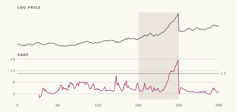

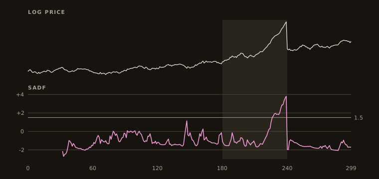
The example's series and its SADF. The shaded span is the run-up.

Before the run-up SADF sits around −1.1, which is what a random walk gives. Inside it the statistic climbs to 3.8 on the last bar before the crash, and it first crosses 1.5 — in the region of the 95% critical values Phillips, Wu and Yu tabulate — at bar 227, thirteen bars before the top. That is late. The run-up had been under way for 47 bars, and detecting explosiveness needs enough of it to have happened.

The Chow-type lines show that test’s assumption at work. On the run-up alone it is emphatic, 8.3. Add the crash and the sixty bars after it and it falls to 1.2 with a break date that means nothing, because the series did not stay explosive. AFML’s §17.4.2 makes this the reason to prefer SADF, which looks at windows ending at each bar and is unaffected by what comes after.

From Rust

use openquant::structural_breaks::{
    get_chow_type_stat, get_sadf, SadfLags, StructuralBreakError,
};

// A log price whose increments compound: explosive by construction.
let mut y = vec![4.0_f64];
for t in 1..120 {
    let wobble = if t % 2 == 0 { 0.002 } else { -0.002 };
    y.push(y[t - 1] + 0.0005 * 1.05_f64.powi(t as i32) + wobble);
}

let sadf = get_sadf(&y, "linear", true, 20, SadfLags::Fixed(1))?;
// One lag uses two leading bars; the first statistic then needs min_length more.
assert_eq!(sadf.len(), y.len() - 2 - 20);
assert!(sadf.last().unwrap() > &3.0);

let chow = get_chow_type_stat(&y, 20)?;
assert_eq!(chow.len(), y.len() - 2 * 20);

// Too short a series is not an error for these two: they return nothing.
assert!(get_chow_type_stat(&y[..30], 20)?.is_empty());
assert!(matches!(
    get_sadf(&y, "cubic", true, 20, SadfLags::Fixed(1)),
    Err(StructuralBreakError::InvalidModel(_))
));

What to watch for

• get_chu_stinchcombe_white_statistics departs from mlfinlab. The CUSUM statistic of §17.3.2 divides a price change by $\hat\sigma_t\sqrt{t-n}$. mlfinlab, and this library before #104, divided by $\hat\sigma_t^{2}\sqrt{t-n}$, so the result depended on the units of the series: on random walks with a 1% step it exceeded its critical value on 94% of bars. It now follows the book and is unchanged by rescaling the series; on the same walks it exceeds the critical value on about 4% of bars at any step size. Since #173 $\hat\sigma_t^2$ is also the book’s mean of the squared differences up to bar $t$; it used to divide their sum by one fewer than their number, which made early statistics slightly small (the one-sided maximum on the test fixture moved from 5.3797 to 5.3921). From Python it returns the tuple (critical_values, statistics), in that order.
• SADF is cubic in the sample length. Every bar refits a regression for every admissible start: $O(n^2)$ regressions of up to $n$ rows. A few hundred bars are quick, a few thousand are slow, and AFML’s §17.4.2.3 puts a full tick history at supercomputer scale. Compute it on sampled bars, cap the look-back by passing a trailing slice, or parallelise over end dates yourself.
• Build the extension with --release before running SADF from Python. maturin develop builds an unoptimised debug extension unless told otherwise, and the many small regressions above are where that shows: a full-series run took about 7.5 minutes per model through a debug build (#77). Use maturin develop --release or just py-develop-release.
• Critical values are not supplied. SADF does not follow a Dickey–Fuller distribution; its critical values depend on the sample length and min_length and come from simulation (Phillips, Shi and Yu, 2015). As a feature this does not matter, since the model learns its own thresholds. As a test, simulate random walks of your length and read off the quantile.
• "quadratic" and the sm_ models changed in #166. Before it, "quadratic" had only the squared trend (no linear $t$), the sm_ models took the supremum of the signed $t$-ratio, so a falling trend scored low, and "sm_power" took $\log 0$ on its first row and silently dropped the windows starting there. Values computed with earlier versions of these four models are not comparable; "linear" is unchanged.
• Time is the row’s position in the whole input, not in the window. It makes no difference to the polynomial and exponential models, whose trend coefficient does not depend on where time starts, but "sm_power"’s $\log t$ does: passing a trailing slice instead of the full history changes its values.
• A window whose regression is singular is skipped, not reported. If every window at a bar is singular — a constant stretch of prices — that bar’s SADF is $-\infty$.
• Detection lags the break. As the example shows, the statistic crosses a threshold well into the episode. It tells you a bubble is under way, not that one is starting.

Related modules

• filters — the CUSUM filter, which samples events and shares only a name with the CUSUM test here.
• fracdiff — the other use of unit-root thinking in this library.
• synthetic-backtesting — relies on a regime holding still; these tests say when it has not.
• feature-importance — to check whether a break statistic earns its place as a feature.

API reference

Python

Signatures, parameters, return values and errors for every function: openquant.structural_breaks.

• structural_breaks.get_sadf — Supremum ADF and sub/super-martingale explosiveness statistics.
• structural_breaks.get_chow_type_stat — Chow-type Dickey-Fuller statistics for a single break at each candidate date.
• structural_breaks.get_chu_stinchcombe_white_statistics — Chu-Stinchcombe-White CUSUM test on levels, with its critical values.

Rust

Rustdoc for this commit, with every public item of openquant::structural_breaks (after a crates.io release the same pages are on docs.rs):

• get_sadf
• get_chow_type_stat
• get_chu_stinchcombe_white_statistics
• SadfLags
• ChuStinchcombeWhiteResult
• StructuralBreakError