Research gallery

SYNTHETIC data

Every committed result on this page is computed on simulated series or on the committed SYNTHETIC sample SYN_A..SYN_E (see DATA_SOURCES.md). None of it describes a real market.

A runbook is a notebook that states a falsifiable hypothesis before it is run, tests it on data where the right answer is known, and ends with a promotion decision: what, if anything, later work should adopt. The notebooks are executed in CI (.github/workflows/notebooks.yml) and committed with their outputs, and this page is rebuilt from those outputs, so each result below is the text the notebook printed or wrote on its last committed run. The hypotheses are quoted in part (the H1, H2, … statements); each runbook’s page and notebook have the full pre-registration, the method and the controls.

#	Runbook	Figures	Decision
09	Fractional differentiation, stationarity versus memory (SYNTHETIC data)	4	Do not promote
10	HRP versus inverse-variance and CLA, out of sample (SYNTHETIC Monte Carlo)	3	Replicated on synthetic data; not promoted as a market claim
11	Triple-barrier labeling and meta-labeling (SYNTHETIC data)	3	Promote the procedure, not a strategy and not the F1 claim
12	CPCV backtest with PSR and the deflated Sharpe ratio (SYNTHETIC data)	3	Promote the evaluation protocol, not a strategy
13	Bet sizing from predicted probabilities (SYNTHETIC data)	3	Promote probability sizing as the default sizing stage after a meta-model that has shown skill. Promote no strategy
14	Fracdiff features against returns in a purged-CV classifier, net of costs (SYNTHETIC data)	3	Do not promote

09 · Fractional differentiation, stationarity versus memory (SYNTHETIC data)

Runbook page · notebook 09_fracdiff_stationarity_memory.ipynb

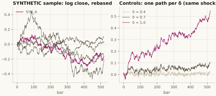
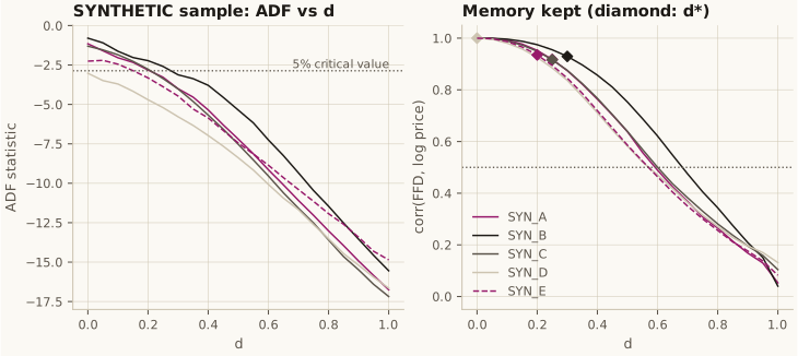
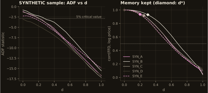
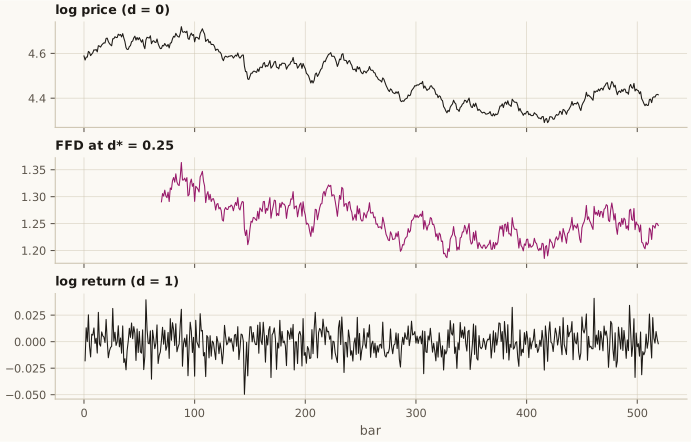
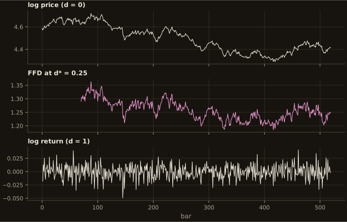
Hypothesis

H1. For each series there is a minimum $d^* < 1$ on the grid at which the fixed-width-window fractionally differenced (FFD) log price rejects a unit root (ADF, constant, one lag, 5%), and at that $d^*$ the FFD series keeps a correlation of at least 0.5 with the original log price (AFML Fig. 5.5 analogue).

Result

As printed by the notebook’s Analysis section:

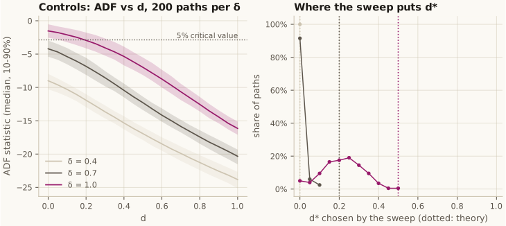
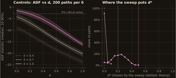
sample symbols supporting H1: 5 of 5
sample d*: [0.25, 0.3, 0.25, 0.0, 0.2]
sample corr at d*: [0.918, 0.929, 0.916, 1.0, 0.935]
sample weight_sum at d*: [0.282, 0.22, 0.282, 1.0, 0.365]
train-half d* passes on the test half: 4 of 5
controls delta=0.4: theory d*=0.0, median d*=0.0, below theory on 0% of paths (0% with 5 lags)
controls delta=0.7: theory d*=0.2, median d*=0.0, below theory on 100% of paths (92% with 5 lags)
controls delta=1.0: theory d*=0.5, median d*=0.2, below theory on 100% of paths (88% with 5 lags)

Promotion decision

Decision: do not promote. Later runbooks should not use “per-symbol $d^*$ = the smallest $d$ passing ADF at 5%” as their default feature transform.

The rest of the decision

H1 passes as it was written, 5 of 5, but the controls with known memory show that passing it does not mean stationarity. On random walks the rule picks $d \approx 0.2$-$0.3$, where theory needs more than 0.5, on 199 of 200 paths. The retained memory is inflated by truncated weights that pass a fifth to a third of the level through, and the selected $d^*$ moves as much between the halves of the sample as it varies between symbols. A feature built this way would be less stationary than the procedure says, and its apparent memory would partly be the price level.

What later runbooks should do instead:

• Keep frac_diff_ffd as a candidate feature, with $d$ chosen on the training span only and reported as a hyperparameter that counts toward the trial total.
• If $d$ is chosen by a test, pair ADF with a test whose null is stationarity (KPSS or similar), or use an estimate of the memory parameter, not the first ADF rejection.
• Report the sum of the truncated FFD weights next to any FFD feature, and lower thresh until it is near 0 when the history allows.
• Settle whether FFD features add predictive value (issue #49’s classifier leg) on real data or on a synthetic series with a planted signal, in purged CV and net of costs. This runbook does not test that.

The decision describes the procedure, established on synthetic series whose memory is known. It says nothing about the $d^*$ of any real instrument. Run the notebook on your own data (see the top cell) and read the controls table next to your own $d^*$ table.

10 · HRP versus inverse-variance and CLA, out of sample (SYNTHETIC Monte Carlo)

Runbook page · notebook 10_hrp_vs_ivp_cla_oos.ipynb

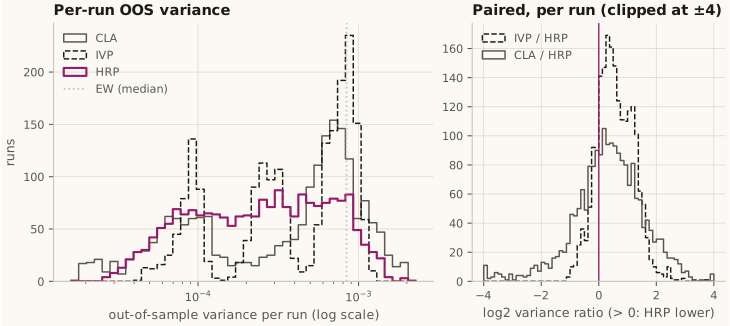
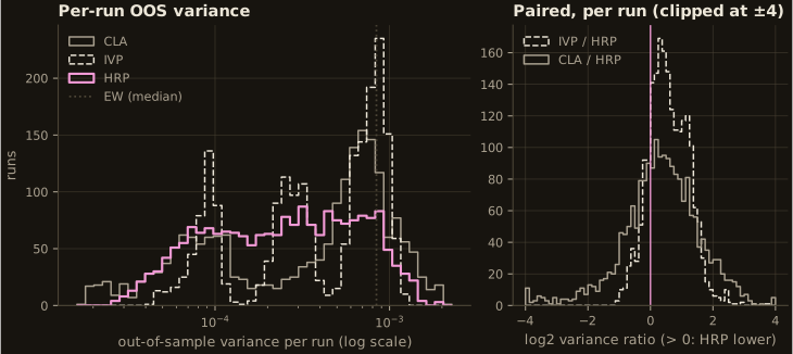
Hypothesis

• H1 (vs CLA). HRP’s OOS variance is lower than that of CLA’s minimum-variance portfolio: the mean of $\log(\sigma^2_{\text{CLA}}/\sigma^2_{\text{HRP}})$ over runs is positive with $t > 1.645$.
• H2 (vs IVP). HRP’s OOS variance is comparable to or lower than inverse-variance weighting: the mean of $\log(\sigma^2_{\text{IVP}}/\sigma^2_{\text{HRP}})$ is not significantly negative ($t > -1.645$).

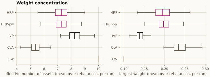
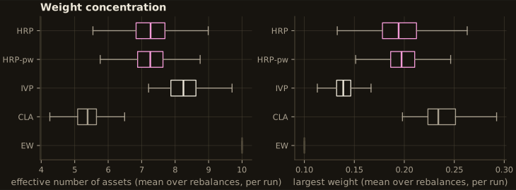
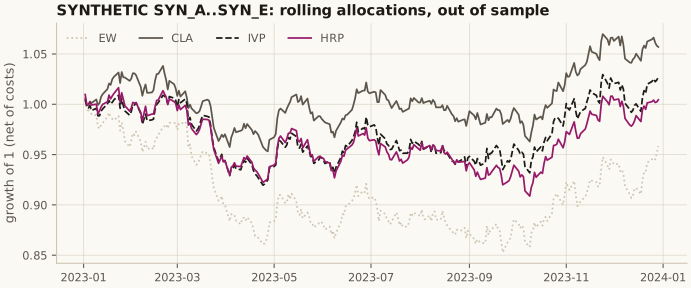
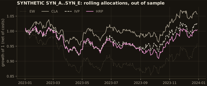
Result

Both hypotheses hold under the Snippet 16.4 process. HRP’s mean OOS variance is about 29% below CLA’s minimum-variance portfolio (ratio 1.40) and 26% below IVP’s (ratio 1.36), and it is lower in 64% and 83% of individual runs. The paired log-ratio $t$-statistics (12.2 and 40.6) leave no doubt about the sign; the effect sizes are what deserve reading. Equal weight, which estimates nothing, has more than twice HRP’s variance, because it always holds a full tenth of every shocked asset.

Promotion decision

Replicated on synthetic data; not promoted as a market claim.

The rest of the decision

• H1 (HRP below CLA minimum variance) and H2 (HRP not worse than IVP) are supported under AFML’s Snippet 16.4 process, in direction. With the book’s tree (the default since #167) the ratio to IVP matches the book’s; the ratio to CLA is smaller than the book reports.
• What this promotes: the hrp and cla bindings reproduce the chapter’s qualitative result, and the runbook is a working template for the same study on real data.
• What it does not: any statement that HRP lowers variance on real assets. That needs the rolling study on a real multi-asset universe (issue #51’s original scope), run with SOURCE set to the user’s own data, net of costs, with its trial count recorded, and it stays open.
• Resolved since: HRP’s turnover above CLA’s was a property of the pairwise tree (#167); HCAA returning HRP’s weights was #108.

11 · Triple-barrier labeling and meta-labeling (SYNTHETIC data)

Runbook page · notebook 11_meta_labeling_triple_barrier.ipynb

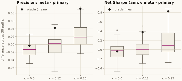
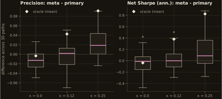
Hypothesis

• H1 (precision). Meta’s precision is higher than primary’s.
• H2 (F1). Meta’s F1 is higher than primary’s. This is the book’s claim (§3.6).
• H3 (risk-adjusted return). Meta’s daily Sharpe ratio net of costs is higher than primary’s.
• H4 (evidence on one path). On the headline path, meta’s deflated Sharpe ratio, deflated by every configuration recorded in the trial registry, is at least 0.95.

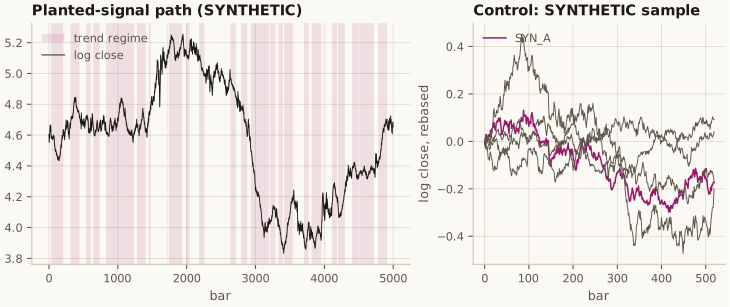
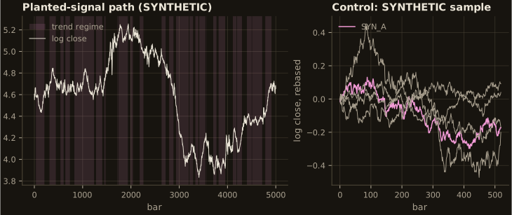
Result

As printed by the notebook’s Analysis section:

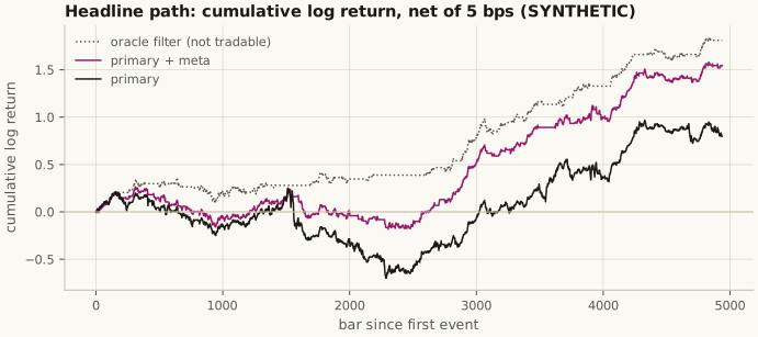
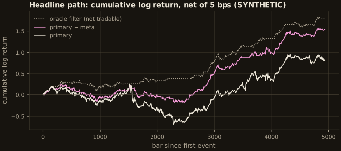
headline path: precision 0.572 -> 0.614 (oracle 0.650); F1 0.728 -> 0.683; net Sharpe (ann.) 0.35 -> 0.78 (oracle 1.27); DSR 0.323 -> 0.924
H1 precision: kappa=0.25 mean diff +0.0217, t = 4.17 -> supported; null kappa=0: t = -3.73 -> control (|t| < 1.96) fails, against meta
H2 F1: kappa=0.25 mean diff -0.0830, t = -11.38 -> rejected; null kappa=0: t = -10.05 -> control (|t| < 1.96) fails, against meta
H3 Sharpe (ann.): kappa=0.25 mean diff +0.1381, t = 2.73 -> supported; null kappa=0: t = -0.70 -> control (|t| < 1.96) passes
H4 (headline-path DSR >= 0.95): rejected (DSR 0.924)
control (SYNTHETIC): meta DSR 0.001 -> passes (no false discovery)

Promotion decision

Decision: promote the procedure, not a strategy and not the F1 claim.

The rest of the decision

Promoted as the default meta-labeling stage for later runbooks that have a primary model:

• triple-barrier meta-labels from the primary model’s side;
• uniqueness-weighted meta-model fitted on training folds only;
• out-of-fold probabilities from purged k-fold, with a walk-forward check;
• every configuration recorded in a TrialRegistry, and the deflated Sharpe ratio read from it.

On data with a known, weak, time-varying edge, this procedure finds part of the edge. It raises precision and the net Sharpe ratio across paths, and it stays below the oracle. On data with no edge it finds nothing: no false discovery on the SYN_* sample, and no Sharpe gain at $\kappa = 0$.

Not promoted:

• Any strategy. The pre-registered strategy’s DSR on the headline path is 0.924, below 0.95. Everything here is synthetic.
• “Meta-labeling improves F1.” It cannot when the primary model takes every bet and is already right more often than not.
• Binary filtering at 0.5 as the sizing rule. Probability sizing did better, post hoc. It should be the pre-registered rule next time, with its own trial count.
• Sequential-bootstrap bagging over the logistic model. It did better on the one headline path, post hoc, and was not run across paths. It is a candidate for a pre-registered comparison.

Conditions for later runbooks that use this stage:

• Judge it on precision and the deflated Sharpe ratio, not F1.
• Run a null (zero-signal simulation, or labels permuted within folds) through the same CV, and compare the precision gain against that null. The per-path comparison is biased against meta-labeling when there is no signal.
• Persist the trial registry (OPENQUANT_RUNBOOK_REGISTRY) across sessions, so the deflation counts every configuration ever tried on that data.

This decision describes the procedure on synthetic series. It says nothing about any real instrument. Run the notebook on your own data (see the top cell) and read the control tables next to your own.

12 · CPCV backtest with PSR and the deflated Sharpe ratio (SYNTHETIC data)

Runbook page · notebook 12_cpcv_deflated_sharpe.ipynb

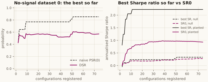
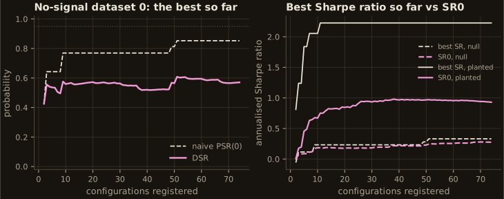
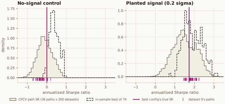
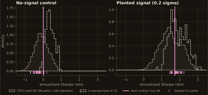
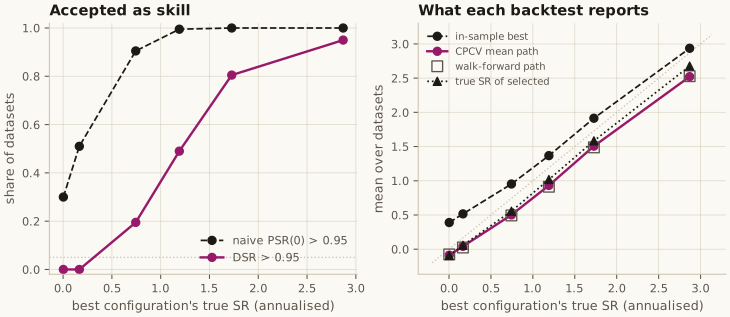
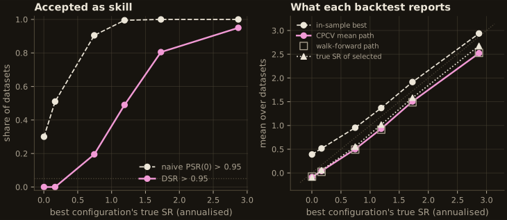
Hypothesis

• H1 (no-signal control: deflation controls false discoveries). When no configuration has an edge, (a) the naive test, PSR(0) > 0.95 on the in-sample best configuration, fires in more than 5% of datasets (exact one-sided binomial test against 5%), and (b) the deflated test, DSR > 0.95 with N = the registry’s trial count, fires in no more than 5% (the same binomial test does not reject 5%).
• H2 (planted weak signal: deflation keeps real discoveries). At the planted strength (drift s.d. 0.2 σ, where the best configuration’s true annualised Sharpe ratio is about 1.7, see Data), DSR > 0.95 in more than half of datasets (exact one-sided binomial test against 50%).

Result

H1 is supported: the naive test finds skill where there is none, and DSR does not. On the no-signal control the in-sample best of 74 has a mean Sharpe ratio of 0.39, while the configuration it picks has a true Sharpe ratio of −0.09. Its PSR(0) clears 0.95 in 30% of datasets (60 of 200) against a nominal 5%. DSR, deflated by the registry’s 74 trials, clears 0.95 in none of them. The deflation figure shows the mechanism on dataset 0: as configurations are added, the best-so-far’s PSR(0) climbs from 0.43 to 0.85 while its DSR stays between 0.5 and 0.6, because SR0, the best that luck alone would reach, rises with the maximum. Dataset 0 happens not to cross 0.95 naively (PSR 0.85); its MinTRL at SR* = 0 is 24.7 years, against the 10 in the sample. The Monte Carlo, not dataset 0, is the evidence.

H2 is supported: DSR keeps a real edge of this size. At the planted strength, where the best configuration’s true Sharpe ratio is 1.73, DSR accepts the in-sample best in 80.5% of datasets (161 of 200). On dataset 0 it accepts outright (DSR 1.00; MinTRL 0.6 years against SR* = 0 and 1.6 years against SR0 = 0.93).

Promotion decision

Promote the evaluation protocol, not a strategy.

The rest of the decision

• Promoted as the default for every strategy-selection runbook: record every configuration in an openquant.evaluation.TrialRegistry before selecting; report the DSR with the registry’s N next to any PSR; report the CPCV mean path Sharpe ratio (or a walk-forward one) rather than the in-sample best; and state MinTRL. On data with a known answer this protocol made no false discovery in 200 no-signal datasets and kept 80% of a true Sharpe ratio of 1.7.
• With two caveats written down: DSR with the raw trial count is conservative when the trials are correlated, so a DSR below 0.95 on a correlated grid is weak evidence of no skill; and the spread of CPCV paths within one dataset is not a confidence interval for the Sharpe ratio.
• Not promoted: the MA-crossover family, which has no edge on the data-layer sample (random walks, as expected). Whether it has one on real data is open. Run this notebook with OPENQUANT_RUNBOOK_SOURCE and a persistent OPENQUANT_RUNBOOK_REGISTRY_DIR to find out.
• Follow-ups worth filing: an effective-number-of-trials estimate (e.g. ONC clusters of trial returns) for TrialRegistry; and a sentence on the backtesting_engine page that path dispersion reflects selection instability, not sampling error.

13 · Bet sizing from predicted probabilities (SYNTHETIC data)

Runbook page · notebook 13_bet_sizing_from_probabilities.ipynb

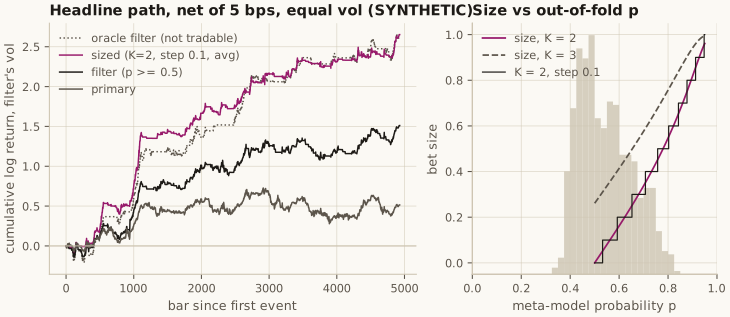
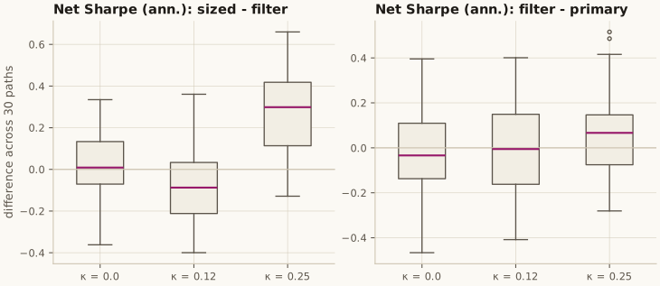
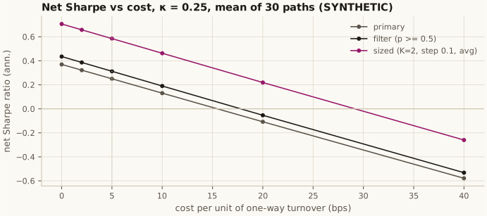
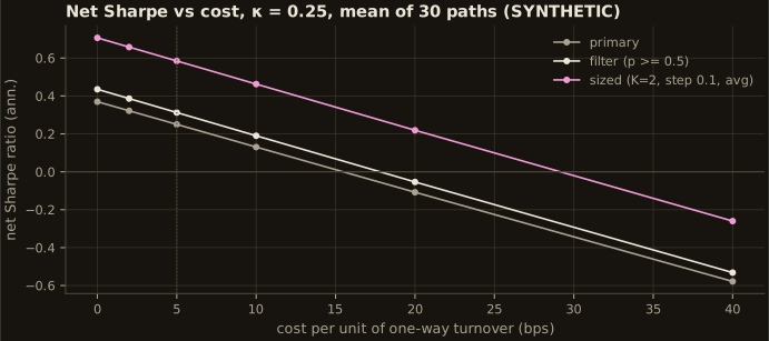
Hypothesis

• H1 (sizing beats filtering). At the headline strength ($\kappa_{\text{trend}} = 0.25$), sized’s annualised net Sharpe ratio is higher than filter’s: paired one-sided $t > 1.645$ over 30 fresh simulated paths.
• H2 (evidence on one path). On a fresh headline path, sized’s deflated Sharpe ratio is at least 0.95, deflated by every configuration evaluated on that path (the trial grid below: 21 configurations, including the number-of-classes, step-size and averaging choices, and configurations that take no bet).
• H3 (no false discovery). Where there is no signal, sizing does not manufacture one:
  • (a) on the zero-signal generator ($\kappa = 0$, 30 paths), sized does not beat filter (paired $t < 1.645$);
  • (b) on the same paths, the best configuration of the 21-trial grid, chosen after the fact on each path, has a DSR of at least 0.95 on no more than 5% of paths (exact one-sided binomial test at 5%: 5 or more of 30 fails);
  • (c) on the SYN_* sample, neither sized nor the best of the grid has a DSR of at least 0.95.

Result

As printed by the notebook’s Analysis section:

headline path, net Sharpe (ann.): primary 0.30, filter 0.78, sized 1.32, oracle filter 1.31
H1 (sized > filter, kappa=0.25): mean diff +0.272, t = 7.03 -> supported
H2 (headline-path sized DSR >= 0.95): supported (DSR 1.000)
H3a (kappa=0, sized not > filter): mean diff +0.011, t = 0.38 -> passes
H3b (kappa=0, best-of-grid DSR >= 0.95 on <= 5% of paths): 0 of 30 (p = 1.000) -> passes
H3c (SYNTHETIC control, sized and best-of-grid DSR < 0.95): sized 0.004, best 0.075 -> passes

Promotion decision

Decision: promote probability sizing as the default sizing stage after a meta-model that has shown skill. Promote no strategy.

The rest of the decision

Promoted, for later runbooks that use runbook 11’s meta-labeling stage:

• Snippet 10.1 with $K$ equal to the meta-model’s number of classes ($K = 2$ for a binary meta-label), floored at zero: follow the primary model or stand aside, never bet against it;
• averaging of live bets (Snippet 10.2) and a step of 0.1 (Snippet 10.3), through bet_sizing.bet_size_probability. On this generator neither choice changed the result, so they are kept for the book’s reasons (fewer flips, fewer small orders), not because they were shown to help;
• every sizing choice ($K$, step, averaging, signed or floored) registered as a trial.

Conditions:

• Gate on skill first. Size by probability only after the meta-model beats the primary model as a filter, judged against a null run (runbook 11’s condition). With a weak signal ($\kappa = 0.12$) sizing did worse than filtering.
• Report break-even cost and exposure next to the Sharpe ratio. The sized book is small, so its Sharpe ratio is reachable only with leverage, and capacity has to be checked against real impact costs.
• Keep reading the DSR over the whole grid. On one path at the headline strength, the sized rule clears 0.95 about a third of the time.

Not promoted:

• Any strategy. Everything here is synthetic, and the planted signal was tuned (in runbook 11) to be detectable.
• $K = 3$ for a binary model, and signed sizing. Both did worse than the headline rule.
• Claims about step size or averaging. This generator has too little overlap between bets to test them.

This decision describes the procedure on synthetic series. It says nothing about any real instrument. Run the notebook on your own data (see the top cell) and read the control tables next to your own.

14 · Fracdiff features against returns in a purged-CV classifier, net of costs (SYNTHETIC data)

Runbook page · notebook 14_fracdiff_features_classifier.ipynb

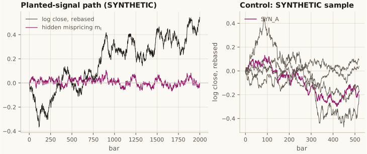
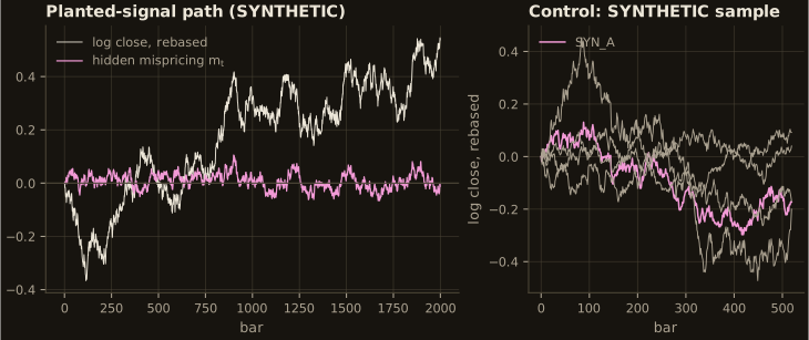
Hypothesis

• H1 (prediction). FFD’s out-of-fold AUC is higher than returns’.
• H2 (net of costs). FFD’s annualised Sharpe ratio net of 5 bps per unit turnover is higher than returns’.
• H3 (against integer differences). FFD’s out-of-fold AUC is higher than the integer differences’.
• H4 (evidence on one path). On the headline path, FFD’s deflated Sharpe ratio, deflated by every configuration recorded in the trial registry, is at least 0.95.

Result

As printed by the notebook’s Analysis section:

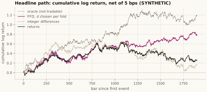
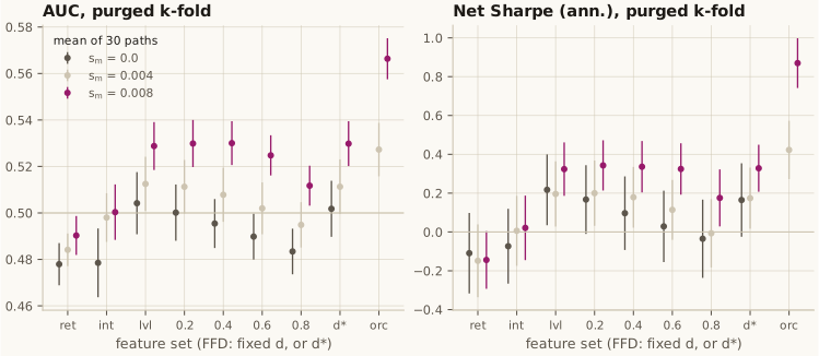
headline path: AUC returns 0.505, int_diff 0.487, FFD 0.530 (oracle 0.572); net Sharpe (ann.) 0.22, 0.13, 0.60 (oracle 0.83)
H1 ffd_dstar - returns: auc: s_m=0.008 mean diff +0.0395, t = 7.44 -> supported; null s_m=0: t = 4.63 -> control fails
H2 ffd_dstar - returns: sharpe_net_ann: s_m=0.008 mean diff +0.4724, t = 6.06 -> supported; null s_m=0: t = 3.35 -> control fails
H3 ffd_dstar - int_diff: auc: s_m=0.008 mean diff +0.0295, t = 4.68 -> supported; null s_m=0: t = 2.90 -> control fails
H4 (headline-path DSR >= 0.95): rejected (DSR 0.779)
control (SYNTHETIC): highest DSR of 8 trials 0.863 -> passes (no false discovery)
pre-registered decision rule: do not promote

Promotion decision

Decision: do not promote. FFD features with $d$ chosen per training fold do not become the default classifier input over returns (or over integer differences).

The rest of the decision

They pass H1-H3 on the planted signal, but the pre-registered null control fails: in purged k-fold CV they beat returns by most of the same margin on random walks. The post hoc walk-forward run shows why: purged k-fold flatters any feature that carries the price level and handicaps returns. Where the signal is real, walk-forward still finds FFD ahead of returns net of costs, but that comparison was not pre-registered, and FFD there did no better than the raw log price.

What later runbooks should do instead:

• Evaluate memory-bearing features walk-forward (cross_validation.walk_forward_splits, added for #217), or with CPCV and a null run through the same splits (cross_validation.null_score_distribution). Purged k-fold removes label overlap, not a model’s knowledge of where the price went after the test fold, and on the SYN_* random walks it gave the level a net Sharpe ratio of 1.85.
• Judge on net returns against a null run, not on pooled out-of-fold AUC, which stayed biased toward memory features even walk-forward.
• Compare FFD with the level, not only with returns. With $d$ chosen by the ADF rule, FFD was the level in all but name here.
• Next runbook (candidate, pre-register it): walk-forward FFD vs returns vs level, net Sharpe ratio, with the zero-signal null through the same splits, on real data.

The decision describes the procedure on synthetic series. It says nothing about FFD features on any real instrument. Run the notebook on your own data (see the top cell) and read the control tables next to your own.

API tours

These notebooks have no pre-registered hypothesis and promotion decision, so they are not runbooks: they show how a few calls fit together on synthetic data and claim nothing (see the notebook contract). They are executed and checked in CI in the same way.

01 · Event labeling and the mid-frequency pipeline

notebook 01_event_labeling_and_pipeline.ipynb

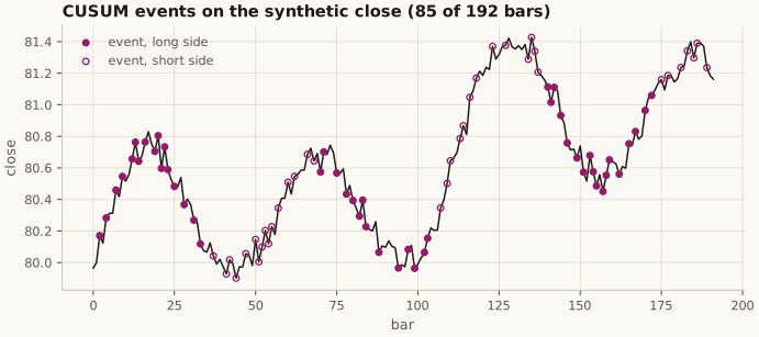
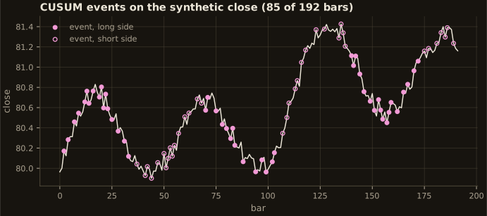
A deterministic synthetic futures dataset (make_synthetic_futures_dataset, seed 7; generated in memory, not market data) run through the AFML-style mid-frequency pipeline: CUSUM event sampling (AFML Ch. 2), side/probability signals (Ch. 3 and 10), portfolio weights (Ch. 16) and risk checks (Ch. 14).

02 · Sequential bootstrap diagnostics

notebook 02_purged_cv_and_seq_bootstrap.ipynb

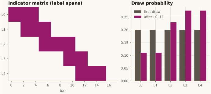
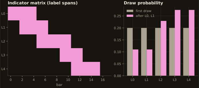
Indicator matrix, average uniqueness and sequential-bootstrap draw probabilities (AFML Ch. 4) on a hand-written set of five overlapping labels.

03 · Feature diagnostics payloads

notebook 03_feature_diagnostics.ipynb

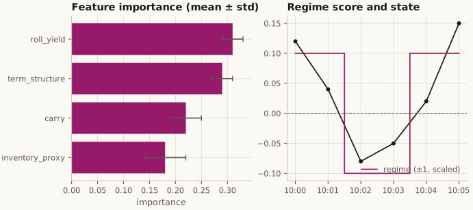
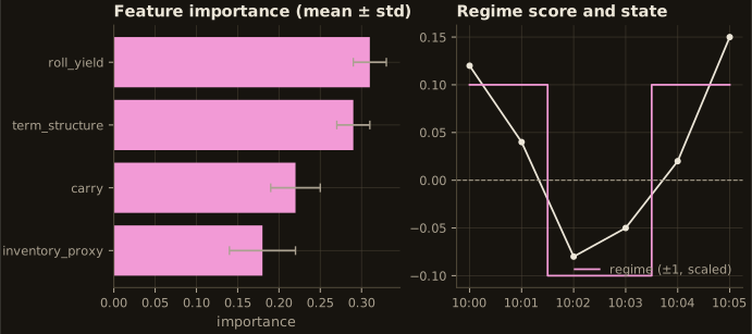
Feature-importance and regime payloads from openquant.viz, rendered with matplotlib. The importance values are illustrative inputs, not the output of a fitted model.

04 · Portfolio construction

notebook 04_portfolio_construction.ipynb

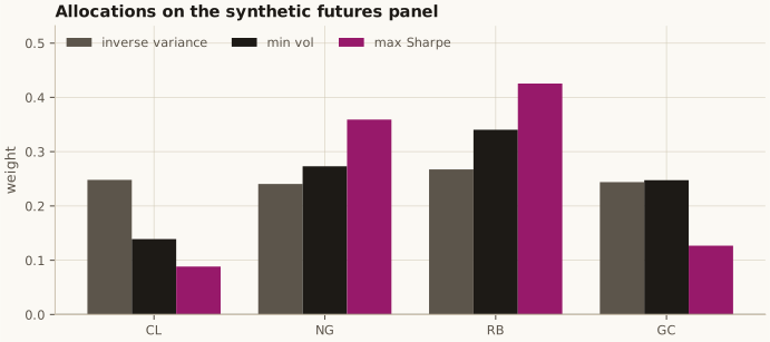
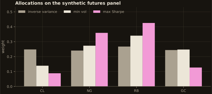
Inverse-variance, minimum-volatility and maximum-Sharpe allocations (AFML Ch. 16 baselines) on the synthetic futures panel (make_synthetic_futures_dataset, seed 9).

05 · Risk overlays and the flywheel’s promotion gates

notebook 05_risk_overlays_and_reality_check.ipynb

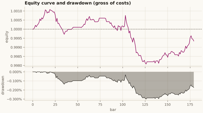
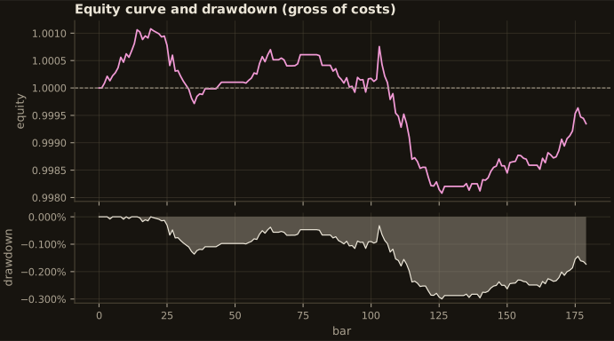
The flywheel’s cost-adjusted promotion gates (realised Sharpe, net Sharpe and leakage guards), on the synthetic futures dataset (seed 13). The equity curve and drawdown come from openquant.viz.prepare_drawdown_payload.

07 · Feature engineering and screening

notebook 07_feature_engineering_discovery_loop.ipynb

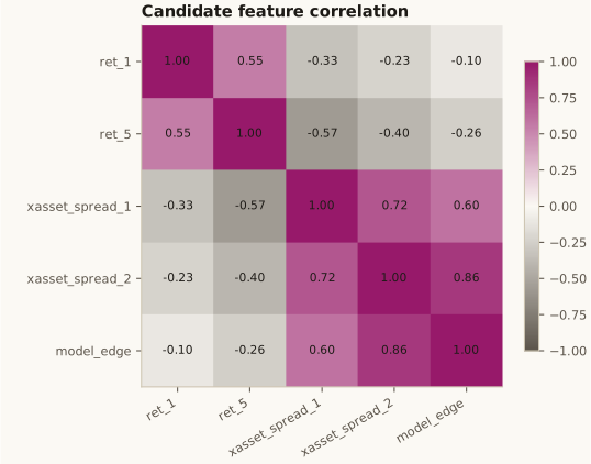
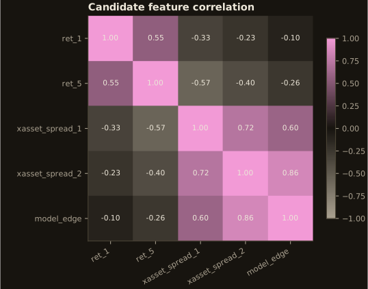
Build candidate features, screen them for basic quality/correlation constraints, and run a quick flywheel check on the synthetic futures dataset (seed 19).

08 · Algo wheel experiments

notebook 08_algo_wheel_experiments.ipynb

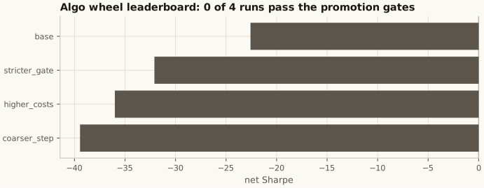
Run a small parameter wheel and rank candidates by net Sharpe and promotion status.