dynamic_allocation

Changing an allocation can consume enough return to change which portfolio is best. AFML Chapter 21 models that cost as proportional to the square root of the weight traded. This concave cost makes the optimization non-convex. For a small enough problem, dynamic_allocation enumerates every permitted portfolio trajectory and returns the one with the highest net Sharpe ratio. It is a CPU reference calculation on a discrete grid.

Use it to inspect a small allocation problem or establish a benchmark for another solver. The forecasts are inputs, not estimates made by this module. The answer is optimal for those forecasts and that grid; it is not evidence of out-of-sample performance.

The grid and the objective

pigeonhole_partitions(K, N) lists allocations of K indivisible units among N assets (Snippet 21.1). all_weights(K, N) divides each partition by K and applies every sign pattern (Snippet 21.2). It removes duplicate vectors caused by sign-flipping zeros, preserving their first occurrence in the book’s order. The resulting set $\Omega$ has weights in multiples of $1/K$ and gross exposure $\sum_n |\omega_n| = 1$.

Short positions are allowed. Net exposure can vary; an all-cash allocation is absent from the search grid. initial_weights=None starts from cash before the first horizon. An explicit initial portfolio need only be finite and have length N; it need not lie on the grid. The standalone scoring functions likewise accept finite off-grid trajectories.

For H horizons, the search scores every sequence in $\Omega^H$:

$$\tau_h = \sum_n c_{h,n}\sqrt{|\omega_{h,n}-\omega_{h-1,n}|}, \qquad \mathrm{SR} = \frac{\sum_h (\mu_h^\top\omega_h-\tau_h)} {\sqrt{\sum_h \omega_h^\top V_h\omega_h}}.$$

means[h], covariances[h] and costs[h] describe one horizon. Costs reduce the numerator; the denominator uses gross-return variance. Variances are summed without cross-horizon covariance terms. There is no annualization or risk-free-rate subtraction. There is also no terminal liquidation cost: only transitions into the supplied horizons are charged. If scores tie, the first trajectory in the book’s product order wins.

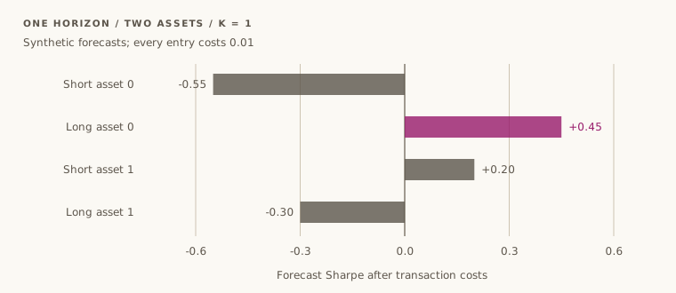
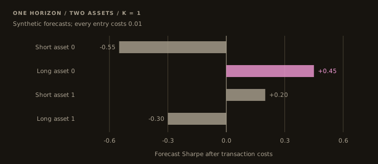
Four candidates, checked individually

With K=1 and two assets, there are only four possible portfolios. The synthetic forecasts below assign returns of 10% and −5%, variance 0.04 to each asset, zero covariance, and cost coefficients of 0.01. Starting from cash, entering any candidate costs 0.01.

from openquant import dynamic_allocation as da

means = [[0.10, -0.05]]
covariances = [[[0.04, 0.0], [0.0, 0.04]]]
costs = [[0.01, 0.01]]
initial = [0.0, 0.0]
print("partitions:", da.pigeonhole_partitions(1, 2))
for weights in da.all_weights(1, 2):
    cost = da.transaction_costs([weights], means, covariances, costs, initial)[0]
    score = da.trajectory_sharpe_ratio([weights], means, covariances, costs, initial)
    print(f"weights={weights}, cost={cost:.2f}, Sharpe={score:.2f}")
best = da.dynamic_optimal_portfolio(means, covariances, costs, k=1)
print("best:", best["weights"])
print(f"net Sharpe: {best['sharpe_ratio']:.2f}")
print("trajectories:", best["trajectories_evaluated"])
try:
    da.dynamic_optimal_portfolio(means, covariances, costs, k=1, max_trajectories=3)
except ValueError as error:
    print("cap:", error)

partitions: [[1, 0], [0, 1]]
weights=[-1.0, 0.0], cost=0.01, Sharpe=-0.55
weights=[1.0, 0.0], cost=0.01, Sharpe=0.45
weights=[0.0, -1.0], cost=0.01, Sharpe=0.20
weights=[0.0, 1.0], cost=0.01, Sharpe=-0.30
best: [[1.0, 0.0]]
net Sharpe: 0.45
trajectories: 4
cap: the search would evaluate 4 trajectories (4 weight vectors over 1 horizons), more than max_trajectories = 3

Long asset 0 wins: $(0.10-0.01)/\sqrt{0.04}=0.45$. Short asset 1 earns a positive forecast return too, but only $(0.05-0.01)/0.2=0.20$. These scores are computed from supplied forecasts, not realized returns.

Every candidate in the one-horizon example, scored by the library after entry costs. Regenerate with python docs-site/scripts/figures/ch21_allocation_figures.py.

Search size is a hard limit

For N=K=3, there are 38 distinct weight vectors. Three horizons require $38^3=54{,}872$ trajectories; five require $38^5=79{,}235{,}168$. The default max_trajectories=1_000_000 admits the former and rejects the latter. The cap is checked before constructing the weight set or scoring trajectories. It is not a time budget or an approximate-search option. Raising it can make a valid request impractical.

Rust’s weight_count(K, N) computes the grid size without constructing the vectors; partition_count(K, N) counts unsigned partitions. Both return None on count overflow. Python exposes neither count helper. len(all_weights(K, N)) is suitable only for small grids because it allocates the entire set; standalone all_weights and pigeonhole_partitions have no trajectory cap.

Calling the API

Python function	Arguments after the function name	Result
pigeonhole_partitions	(k, n)	Integer partitions
all_weights	(k, n)	Distinct signed weight vectors
transaction_costs	(trajectory, means, covariances, costs, initial_weights)	One cost per horizon
trajectory_sharpe_ratio	(trajectory, means, covariances, costs, initial_weights)	Net trajectory Sharpe
dynamic_optimal_portfolio	(means, covariances, costs, k=None, initial_weights=None, max_trajectories=1_000_000)	Dictionary of weights, net Sharpe, costs and count

k=None uses N. Results store weights[h][n], one asset vector per horizon; this is the transpose of the book’s returned array. Inputs must have matching horizon and asset dimensions, finite numbers, non-negative costs, and symmetric positive definite covariance matrices. A singular covariance is rejected even if a particular portfolio would have positive variance. Validation uses a tolerance of 1e-12 times the largest absolute matrix entry for symmetry and squared Cholesky pivots; a sufficiently ill-conditioned matrix can therefore fail too. Scoring an all-zero trajectory fails because its variance is zero. Rust reports DynamicAllocationError; Python maps core validation failures to ValueError. The Python search releases the GIL.

In Rust, forecasts and configuration are explicit structs:

use nalgebra::DMatrix;
use openquant::dynamic_allocation::{
    dynamic_optimal_portfolio, weight_count, DynamicAllocationConfig, HorizonForecast,
};

let horizon = HorizonForecast {
    mean: vec![0.10, -0.05],
    covariance: DMatrix::from_diagonal_element(2, 2, 0.04),
    cost: vec![0.01, 0.01],
};
let result = dynamic_optimal_portfolio(&[horizon], &DynamicAllocationConfig::new(1)).unwrap();
assert_eq!(weight_count(1, 2), Some(4));
assert_eq!(result.weights, vec![vec![1.0, 0.0]]);
assert_eq!(result.trajectories_evaluated, 4);
assert!((result.sharpe_ratio - 0.45).abs() < 1e-12);

Where this fits

combinatorial_optimization supplies generic integer search and a different, single-instrument inventory objective with linear impact and fixed ticket costs. It does not implement this portfolio Sharpe objective. portfolio covers single-period allocation methods.

Implementation references: Rust search and validation and Python binding contract.

API reference

Python

Signatures, parameters, return values and errors for every function: openquant.dynamic_allocation.

• dynamic_allocation.pigeonhole_partitions — Every way to place `k` indivisible units of capital into `n` assets (AFML Snippet 21.1).
• dynamic_allocation.all_weights — The set of signed weight vectors searched by the dynamic allocation (AFML Snippet 21.2).
• dynamic_allocation.transaction_costs — Transaction cost of each horizon of a weight trajectory (AFML Snippet 21.3, `evalTCosts`).
• dynamic_allocation.trajectory_sharpe_ratio — Sharpe ratio of a weight trajectory net of transaction costs (AFML Snippet 21.3, `evalSR`).
• dynamic_allocation.dynamic_optimal_portfolio — Best weight trajectory by exhaustive integer search (AFML Snippet 21.3, `dynOptPort`).

Rust

Rustdoc for this commit, with every public item of openquant::dynamic_allocation (after a crates.io release the same pages are on docs.rs):

• pigeonhole_partitions
• partition_count
• all_weights
• weight_count
• transaction_costs
• trajectory_sharpe_ratio
• dynamic_optimal_portfolio
• HorizonForecast
• DynamicAllocationConfig
• DynamicAllocation