Runbook: triple-barrier labeling and meta-labeling

SYNTHETIC data

Every number and figure on this page comes from simulated price paths with a planted, documented signal, or from the committed SYNTHETIC sample SYN_A..SYN_E (seeded random walks, see DATA_SOURCES.md). None of it describes a real market. Read it as a description of what the procedure does on data where the right answer is known.

Notebook: notebooks/python/11_meta_labeling_triple_barrier.ipynb, committed with its outputs and executed in CI by just notebooks-run. It replaces notebook 06. Module background: labeling, sample_weights, cross_validation, bet_sizing, evaluation.

Why a planted signal

The SYN_* sample is made of random walks, so no primary model has an edge on it. On that sample, “does meta-labeling help?” can only be answered “no”, and a “yes” would mean a bug. So the main study simulates paths where the answer is known in advance:

• Two hidden regimes, each lasting 100 days on average.
• Trend regime. Returns continue the last 20 days’ move: $\kappa = 0.25$ times the day’s volatility, scaled by how large the move was. Daily volatility is 0.7%.
• Chop regime. Returns partly reverse that move ($\kappa = -0.10$). Daily volatility is 1.4%.
• Imperfect proxy. Volatility carries AR(1) noise, so it only partly reveals the regime.

A 10/40-day moving-average crossover makes money in trend, loses it in chop, and has a small edge overall. An oracle filter that knows the regime shows the most any filter could add. Two controls, where the right answer is “no improvement”:

• the same generator with $\kappa = 0$;
• the SYN_* sample, which is also what fetch() returns by default, and what you replace with your own data.

The prototype runs raised the generator’s strength before the notebook was written, from $\kappa = 0.06$ through 0.12 and 0.20 to 0.25, because weaker signals gave no detectable effect. The notebook discloses this, and keeps $\kappa = 0.12$ in its Monte Carlo.

Hypotheses (pre-registered)

Each is tested one-sided at 5%, paired over 30 simulated paths at $\kappa = 0.25$.

• Meta: the logistic meta-model on three features, with out-of-fold probabilities from purged 5-fold CV; it takes a bet when $p \ge 0.5$.
• Primary: takes every bet the crossover proposes.

	Claim	Result
H1	Meta’s precision is higher than primary’s	supported: 0.543 → 0.565, $t$ = 4.2 (walk-forward: +0.018, $t$ = 4.3)
H2	Meta’s F1 is higher than primary’s (AFML §3.6)	rejected: 0.704 → 0.621, $t$ = −11
H3	Meta’s net Sharpe ratio is higher than primary’s	supported: 0.18 → 0.32 annualised, $t$ = 2.7
H4	On the headline path, meta’s DSR over all 10 registered trials is at least 0.95	rejected: DSR 0.924 (0.862 with the 2 post hoc bagging trials)

Method

Per series, following the book:

1. Daily volatility. volatility.get_daily_vol (Snippet 3.1).
2. Events. A CUSUM filter whose threshold is 2 × the volatility known the day before (Snippet 2.4): filters.cusum_filter_indices with one threshold per bar.
3. Primary side. The crossover’s side at the event bar.
4. Meta-labels. Triple barrier at ±1.5 × volatility with a 14-day vertical barrier, using labeling.add_vertical_barrier, triple_barrier_events and get_bins (Snippets 3.2-3.7).
5. Features. Past-only: the volatility ratio, the 20-day efficiency ratio and the MA gap.
6. Weights. Average uniqueness from sampling.get_av_uniqueness_from_triple_barrier.
7. Meta-model. An L2 logistic regression in numpy. scikit-learn is not a dependency, and none was added. Features are standardised on the training fold only, and out-of-fold probabilities come from cross_validation.purged_kfold_splits(t0, t1, 5, pct_embargo=0.01).
8. Positions and returns. bet_sizing.avg_active_signals averages concurrent bets into a position, held from one close to the next. Returns are net of 5 bps per unit of one-way turnover.
9. Evaluation. evaluation.meta_label_metrics gives precision, recall and F1, and evaluation.probabilistic_sharpe_ratio the PSR. The DSR is deflated by every configuration recorded in an evaluation.TrialRegistry.

Trial count. 10 pre-registered configurations on the headline path, all in the registry, and H4’s DSR deflates by all 10:

• the CUSUM multiples 1.0 (the first prototype) and 2.0;
• the primary model;
• binary filters at 0.5 and 0.55 and probability sizing, each on all three features and on the volatility ratio alone;
• the headline rule run walk-forward.

Two more were added after the pre-registered run (#187): the headline rule and probability sizing with sequential-bootstrap bagging as the meta-model. They are recorded in the registry as well, so it holds 12 trials, and H4 is also reported deflated by all 12. A configuration that takes no bet (one on the control) is recorded by TrialRegistry.record with a Sharpe ratio of 0, so it still counts. The Monte Carlo paths describe the method and are not trials.

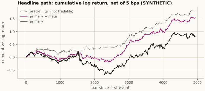
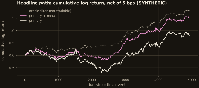
Results (SYNTHETIC)

Headline path (5,000 bars, 708 events):

Strategy	Bets	Precision	Recall	F1	Net Sharpe (ann.)	PSR	DSR
Primary (crossover, every bet)	708	0.572	1.000	0.728	0.35	0.939	0.323
Primary + meta (pre-registered)	508	0.614	0.770	0.683	0.78	1.000	0.924
Oracle filter (not tradable)	369	0.650	0.593	0.620	1.27	1.000	—

Headline path, net of costs. The oracle is the ceiling a perfect regime filter would reach.

Monte Carlo, 30 paths per strength (difference from primary, annualised Sharpe ratio):

$\kappa_{\text{trend}}$	Precision: meta	Precision: oracle	Net Sharpe: meta	Net Sharpe: oracle
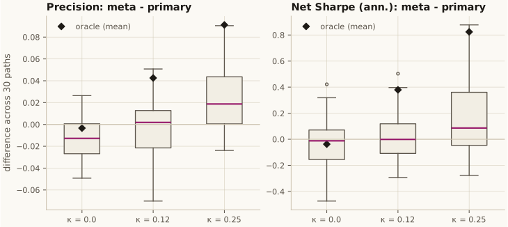
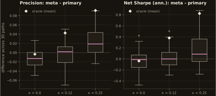
0 (no signal)	−0.014 ($t$ = −3.7)	−0.003	−0.03 ($t$ = −0.7)	−0.04
0.12	−0.003 ($t$ = −0.5)	+0.043	+0.03 ($t$ = 0.7)	+0.38
0.25	+0.022 ($t$ = 4.2)	+0.091	+0.14 ($t$ = 2.7)	+0.82

Gain of meta-labeling over the primary model per path, with the oracle's mean gain as a diamond.

Control on the SYN_* sample:

• The crossover has no edge: precision 0.449, net Sharpe ratio −0.60.
• The meta-model rejects 88% of its bets.
• Meta’s DSR is 0.001 over the same 10-configuration grid, and over all 12. There is no false discovery.

Post hoc: sequential-bootstrap bagging as the meta-model (#187, added after the pre-registered run; a comparison, not a test). sb_bagging.SequentiallyBootstrappedBaggingClassifier (20 mean-threshold stumps, each on a sequential bootstrap sample of 20% of the training events, weighted by uniqueness) is fitted on the same purged folds and features. Its probability is the share of stumps voting 1. DSRs are over all 12 registered trials.

Data	Meta-model	Rule	Bets	Precision	Net Sharpe (ann.)	DSR
Headline path	logistic	binary@0.5	508	0.614	0.78	0.862
Headline path	logistic	sized	508	0.614	1.28	1.000
Headline path	bagging	binary@0.5	334	0.680	1.14	0.996
Headline path	bagging	sized	279	0.710	1.44	1.000
SYN_* control	logistic	binary@0.5	37	0.297	−1.50	0.001
SYN_* control	bagging	binary@0.5	180	0.456	−0.76	0.028

On the headline path the two models’ probabilities correlate at 0.83 and agree on 74% of take/skip decisions; bagging is more selective and more precise. On the control it keeps more of the losing bets but finds nothing. This is one path: bagging is not in the Monte Carlo, because the sequential draw rescans the indicator matrix for every sampled event.

What it means

• Meta-labeling finds part of a real edge and invents none. It recovers about a quarter of the oracle’s precision gain and a sixth of its Sharpe gain. At $\kappa = 0.12$ the oracle still gains on every path, but meta gains nothing: with about 550 training events it needs a large conditional edge.
• F1 is the wrong yardstick here. The primary model takes every bet, so its recall is 1 and its F1 is $2b/(1+b)$ at base rate $b$. A filter that gives up 30% of recall for 2 points of precision lowers F1 even while it raises the Sharpe ratio.
• One path is not enough. On the headline path, 19 years of a 0.78 Sharpe ratio still has a DSR of 0.924 once 10 tried configurations are counted, and 0.862 once the 2 post hoc bagging trials are counted too.
• Precision comparisons are biased against meta when there is nothing to find. On the zero-signal generator, meta’s precision is lower than primary’s ($t$ = −3.7). This is not a leak: a test that replaces the test fold with noise leaves every fitted model bit-identical. It is how leave-fold-out CV behaves. A fold with a high win rate leaves a training set with a low one, so the model takes fewer of that fold’s bets; the correlation is −0.76. So read a precision gain against a null run, not against zero.
• Post hoc: probability sizing did best. Snippet 10.1 sizing had the best Sharpe ratio of the pre-registered configurations on the headline path (1.28, DSR 1.000) and in the Monte Carlo (+0.36, $t$ = 6.1). It also lost more under the null. It was not pre-registered, so it is the candidate for the next study.
• Post hoc: bagging looked better on one path. Sequential-bootstrap bagging raised precision to 0.680 and the net Sharpe ratio to 1.14 (1.44 sized, the best of all 12 trials) on the headline path, and found nothing on the control. One path and two configurations picked after the fact make it a candidate for a pre-registered comparison across paths, not a finding. No pre-registered outcome changes.

Decision

Promote the procedure, not a strategy and not the F1 claim. Later runbooks with a primary model should use this stage:

• triple-barrier meta-labels and uniqueness weights;
• purged k-fold with a walk-forward check;
• every configuration in a TrialRegistry.

They should judge it on precision and the deflated Sharpe ratio, and compare against a null run through the same CV. Sequential-bootstrap bagging is not promoted over the logistic model: it was compared on one path, post hoc. None of this is a claim about any real instrument.

Checks

The notebook asserts all four:

1. Features, sides, volatility and events do not change when the future after a cut is replaced.
2. Labels do not change when closes after $t_1$ change, and do change when closes inside the span change.
3. Purged folds have zero train/test overlaps, and no embargoed event is trained on.
4. A fold’s fitted model is bit-identical when its test fold is replaced with noise.

Audit: features with memory (#217)

Runbook 14 found that purged k-fold, which also fits a middle fold’s model on the events after it, flatters features with memory even on random walks (cross_validation). The meta-model’s features are slowly varying, so this runbook was checked. The zero-signal paths are already a null through the same splits, and the audit added a walk-forward Sharpe comparison to the Monte Carlo. Under the null meta gains nothing in either scheme (k-fold −0.03, $t$ = −0.7; walk-forward −0.01, $t$ = −0.3). With the signal the walk-forward gain is smaller but still clear (+0.08, $t$ = 2.3, against +0.14, $t$ = 2.7). No conclusion changes.

Run it on your own data

The control study reads three environment variables. The planted-signal study does not depend on the data source. Write the executed copy and figures outside the repository:

OPENQUANT_RUNBOOK_SOURCE=/path/to/daily_ohlcv.parquet \
OPENQUANT_RUNBOOK_SYMBOLS=ES,NQ,CL \
OPENQUANT_RUNBOOK_RANGE=2010-01-01:2024-12-31 \
OPENQUANT_RUNBOOK_REGISTRY=$HOME/.openquant/trials-meta-labeling.json \
OPENQUANT_FIGURE_DIR=/tmp/meta-labeling-figures \
  uv run --python .venv/bin/python python notebooks/python/scripts/execute_notebook_cells.py \
    notebooks/python/11_meta_labeling_triple_barrier.ipynb --out /tmp/11_on_my_data.ipynb

OPENQUANT_RUNBOOK_REGISTRY keeps the trial registry between sessions, so every configuration you try on your data counts toward the deflated Sharpe ratio. For a vendor API, set SOURCE in the notebook’s parameters cell to an openquant.data.CallableSource.